Simple Multimodal Design Recommender

In the last post I discussed ways to evaluate the performance of recommender systems. In my experience, there is almost nothing as important, when building recommender and predictive models, as correctly evaluating their quality and performance. You could spend hours in preparing the training data, feature engineering and choosing the most advanced algorithm. But it’s all worth nothing if you can’t tell whether your model will actually work or not, i.e. positively influence your KPIs and business processes.

While researching how to implement recommender systems in Python I came across a really interesting and simple example of a recommender published by Yhat: http://docs.yhathq.com/scienceops/deploying-models/examples/python/deploy-a-beer-recommender.html

Yhat offers a service which allows for easy deploying a recommender without having to worry about scalability and server provisioning. The process of deploying a new recommender to Yhat and putting it into production is very simple, if you’re interested I would encourage you to read more about it here: https://yhathq.com/products/scienceops

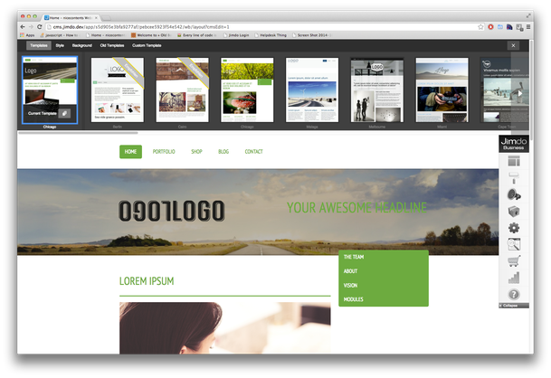
The basis for this demo is an item-to-item similarity matrix. This is being used in order to calculate item recommendations online. I adapted this approach for developing a design recommender at Jimdo. Jimdo is an online website creation and hosting service. At Jimdo we allow our uses to choose from many different designs (as can be seen in the image above) and choosing the right design can be quite time consuming. So we thought of developing a design recommender which would recommend designs to a specific user. The aim is that the user needs less time to find a design that she likes and spends more time adding content.

Following Yhat’s beer recommender example (and that of most item-to-item-recommenders) one would only calculate the similarities for items that could potentially end up in the recommended list of items (in our case the similarities between specific designs). In addition to that, we included attributes that wouldn’t be included in a ranked list, but might be good input-variables/covariates for predicting design-usage behavior. In our case these variables were 1.) whether a user has a free, pro or business account (our three different packages), 2.) which platform language someone chose. 

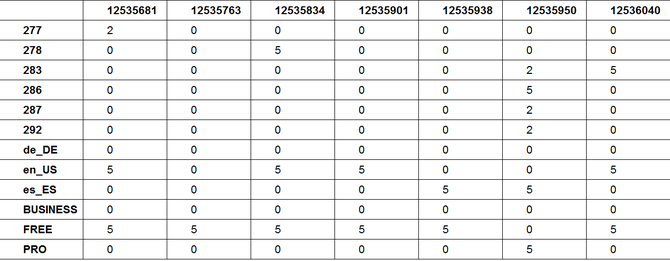
The basis data structure is an affinity table (see below), containing an affinity score for every user towards each of the items and variables. Every column depicts a users affinities. 5 is the highest affinity (user has that language setting, package or has eventually chosen that design), 0 means user has no affinity towards that item or attribute and 2 means she has previewed a design but not chosen it. Since in our case the rating is implicit, meaning the user didn’t give a rating on a five-star-scale, the definition of these affinity values can be seen as part of the feature engineering step. The rows in the affinity table are the specific items and attributes.

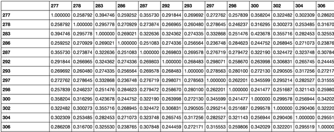
On the basis of this affinity table (df_train) the similarity (in this case cosine-similarity) for every item and attribute to any other item and attribute is calculated with one simple python statement: 

dists = sklearn.metrics.pairwise.cosine_similarity(df_train)

The result of this is the following distance matrix (dists):

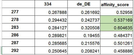
Since the aim is to only recommend design ids (the three digit ids in this case), we cut out all the rows for the attributes we’ve included in the similarity calculation (language, package) but keep the respective columns. To recommend a list of ranked items to a specific user, we would take the input vector of a user, which language setting and package she has and which design she has already seen. For example the following user has language setting de_DE (German) and has previewed the design with id 334. We calculate the affinity score towards each design by summing the item similarities over the two input columns. Then we can rank the items by the resulting affinity score, thereby producing a ranked list of the top-n designs, excluding the designs a user has already seen. (By the way, summing up the two cosine-similarities assumes that there is an additive relationship between those similarities. This might not be the case. Having robust evaluation criteria in place is important when such assumptions are made.)

The Python code for this looks as follows:

def get_top_2(products):

    p = dists[products].apply(lambda row: np.sum(row), axis=1)

    p = p.order(ascending=False)

    return p.index[p.index.isin(products)==False][:2]

print get_top_2(["334","de_DE"])

→ Index([u'283', u'278'], dtype='object')

In this case Design-ID 283 and Design-ID 278 would be recommended in that order if we were to recommend the top-2 items for this specific user. 

As discussed in the last post about evaluating recommender systems the above steps to produce the similarity matrix would all be carried out on the training set of users. We would then evaluate the performance of this specific recommender by producing recommendations on the test set, i.e. users who haven’t been included in calculating the similarity matrix. For example we could take the first designs that a user from the test set has seen, add her language setting and package and use that as the input vector for our recommender, recommend top-3 designs and measure DCG and MAP (read this blog post for details). Then we do the same but produce the top-3 designs by randomly picking 3 design-ids (excluding the ones the user has already seen) and measure DCG and MAP. The improvement against this random-baseline is what should really matter, in our case we had a more than 2-fold improvement on MAP. We could then further modify our recommender, for example by choosing a different similarity-measure (euclidian-distance, log-likelihood-ratio), by playing around with the implicit rating or adding or removing attributes. The aim of this would be to optimize the improvement compared to the random-baseline.

This offline evaluation of the recommender would be followed by an online evaluation through a split-test. It’s important to know what you want to optimize for, especially if the setting isn’t straight forward. In our case we want to make sure that the user doesn’t waste all her time and energy on finding a suitable design. We know that it is critical that a user starts adding content as soon as possible for increasing our user CLV. So in this case the OEC  (overall evaluation criteria) for this split-test would be “time needed to choose a design”.